Basic 2D example

This example (along with all tutorial comments) can be found in examples/basic_ex_2d.py.

If Planktos is properly installed according to the quickstart instructions, loading the library is as easy as:

import planktos

If this fails, Planktos has not been installed. Please follow the installation instructions in the quickstart. Alternatively, you can explicitly specify the location of the planktos library. Depending on where your Planktos script is located, you would need to add the location of the planktos library to your Python path. For instance, assuming that you are within the examples directory, you’d need to start with:

import sys
sys.path.append('..')
import planktos

Once planktos is imported, the first thing we do is create an environment. The default environment is a 10 meter by 10 meter 2D rectangle in which agents can exit out of any side (after which they cease to be simulated). The fluid velocity is zero everywhere until you set it to something else. See the documentation of the environment class in planktos/environment.py for all the options!

envir = planktos.environment()

Let’s add some fluid velocity. First, we’ll specify some (currently unrealistic) properties of our fluid:

envir.rho = 1000 # fluid density
envir.mu = 1000 # dynamic viscosity

Now let’s specify some Brinkman flow. See the documentation for set_brinkman_flow in for information on each of these fluid parameters.

envir.set_brinkman_flow(alpha=66, h_p=1.5, U=1, dpdx=1, res=101)

Since this is a 2D fluid field, we can quickly visualize it to make sure everything looks right. Again, see documentation for options:

envir.plot_flow()

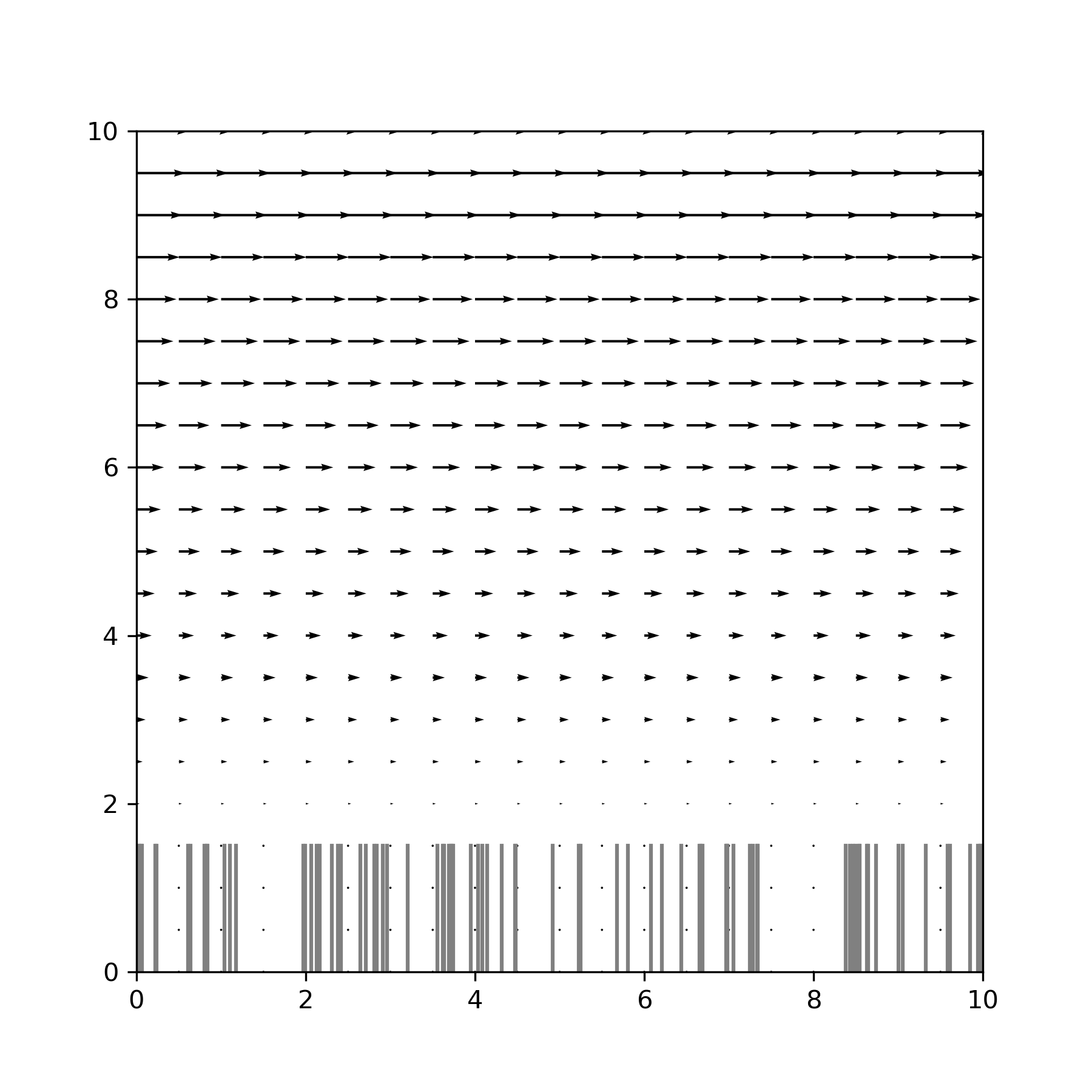
We could also plot vorticity with envir.plot_2D_vort(), but it wouldn’t look like much.

Now, let’s add an agent swarm! Since this is a simple example, we will go with the default agent behavior: fluid advection with brownian motion, or “jitter”. By default, the swarm class creates a swarm with 100 agents initialized to random positions throughout the environment. We just need to tell it what environment it should go in by passing in our environment object:

swrm = planktos.swarm(envir=envir)

Let’s plot our new agents to see what we have so far, with fluid velocity arrows in the background:

swrm.plot(fluid='quiver')

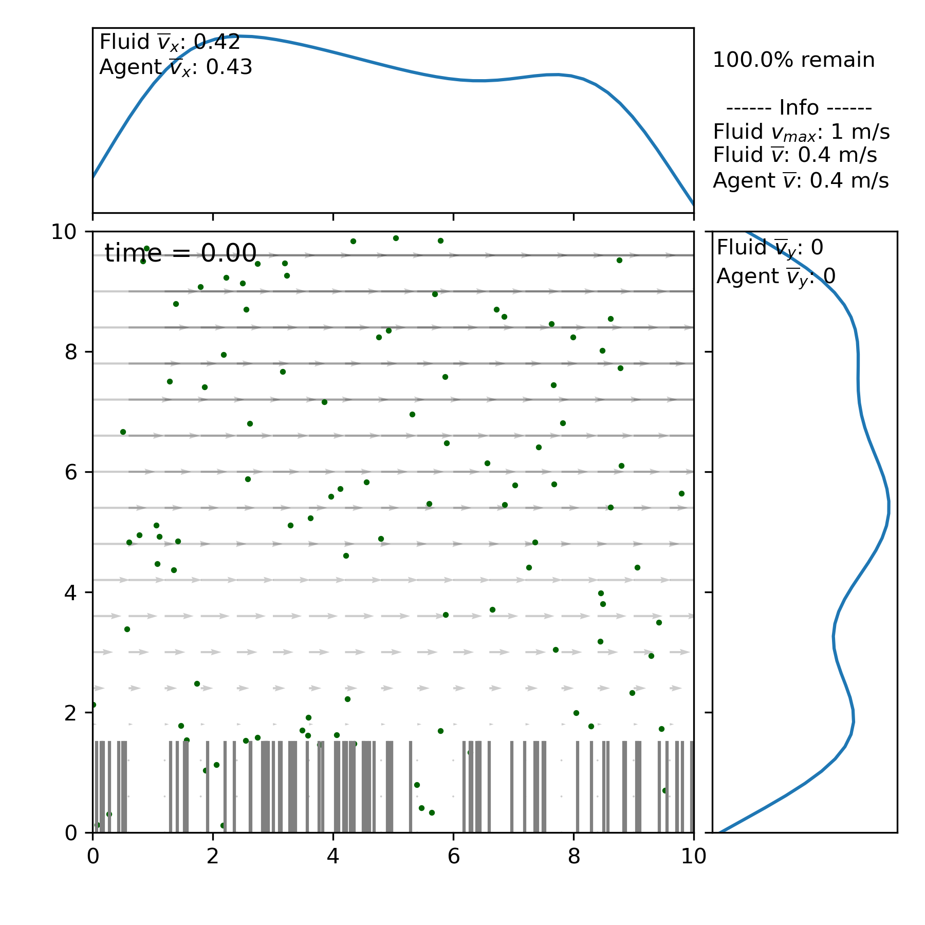
The bars that you see at the bottom denote the height of the porous layer and aren’t really “there” in the sense that the porous layer is homogenous - Planktos just gives them a random distribution to mimic seagrass. To the top and right, you can see the Gaussian kernel density estimation for the swarm. Various statistics are also given.

By default, the swarm is set up with two properties that are the same across all agents: ‘mu’ and ‘cov’. These are the mean drift (not counting the fluid) and covariance matrix for the brownian motion. ‘mu’ defaults to a vector of zeros and ‘cov’ to an identity matrix. Since we are working in units of meters, that’s quite a lot of jitter! Let’s slow those down by editing that property:

swrm.shared_props['cov'] = swrm.shared_props['cov'] * 0.01

It is also possible to set properties which are different between agents. For that, you edit the columns of swrm.props, which is a pandas DataFrame.

Now it’s time to simulate our swarm’s movement! We do this by calling the “move” method of the swarm object in a for loop. “move” takes one argument, which is the temporal step size. For example, if we want to move the swarm for 24 seconds with a step size of 0.1 seconds each time, we use:

for ii in range(240):
    swrm.move(0.1)

We can see where we ended up with swrm.plot(), or we can plot a particular time by calling swarm.plot(time), e.g. swarm.plot(19.1). Or we can just plot everything as a movie with swrm.plot_all(). Run the corresponding example, basic_ex_2d.py in the examples folder to see this animation!

Like many functions in Planktos, plot_all has a lot of options as well. For example, you can generate an mp4 instead of viewing the movie directly by passing in a filename. You can always continue to move the swarm, even after it has already moved. And data about the swarm can be exported using the swrm.save_data function, or swrm.save_pos_to_csv if you only want the positions over time, or swrm.save_pos_to_vtk if you want to visualize the swarm in something like VisIt.

Finally, for the ultimate in interactive usage, open an ipython session and run the basic_ex_2d.py example using the magic command %run:

%run basic_ex_2d.py

After it finishes running, you can interact with both the envir and swrm objects we just created by directly calling functions on them! This can be a useful way to see what kind of commands are available too. For instance, try typing

swrm.

(with the period) but instead of hitting enter, hit tab. A list of attributes and functions should appear. If you choose a function and then add a ? afterward, e.g.:

swrm.plot?

The docstring will appear to give you help on what that function does and how it works. Similarly, Jupyter notebooks are another great way to explore Planktos!